Speed ​​of execution of the first repetition in a series

Speed of execution of the first repetition in a series

In this article, the importance of the execution speed of the first repetition for the dosage, control and evaluation of strength training is exposed in an orderly manner in order to give the opportunity to become aware of the repercussion of the appropriate application of this variable in the development of everything related to strength training.

In this series of articles we deal with some of the most important concepts of strength training, collecting notes from the recently published book Strength, Speed ​​and Physical and Sports Performance written by renowned researchers Juan José González Badillo and Juan Ribas Serna.

SUMMARY

• Speed ​​control comes to overcome the series of inconveniences presented by the use of RM and XRM or nRM in the dosage of training and in the evaluation of its effect.
• It has been confirmed that each percentage of 1RM has its own speed for each exercise. This speed is very stable for the same person when their performance changes, and very similar between people, even when the level of performance between people is very different.
• If the average or average maximum propulsive velocity with which a mass displaces can be measured, by applying these equations we can obtain the percentage of the RM that said mass represents.
• The speed of the first repetition of the series serves to determine with what relative load the subject is training, as well as to determine what has been, and continues to be, the effect of training each day, what has been the evolution of the maximum intensity used every day, and what has been the pre-post training effect…
• The speed with each percentage is very similar between people with a very different level of performance.

 

Indeed, faced with all these inconveniences, it is necessary to find an appropriate solution. If the training schedule is nothing more than the expression of a series or ordered succession of efforts that are dependent on each other, and the effort is the actual degree of demand in relation to the current possibilities of the subject, which represents the nature of the effort, the appropriate solution will be to be able to measure with high precision the character of the effort. This is achieved if it is known:

• The Degree of Effort that represents the first repetition of a series.
• The Degree of Effort that represents the loss of speed within the series.

This article will deal with these two factors as key elements of the quantification, dosage, control and evaluation of the training load and its effects.

The speed with each percentage of the RM and its stability. Degree of Effort that represents the first repetition of a series

A few years ago Professor González-Badillo wrote: “if we could measure the maximum speed of movements every day and with immediate information, this would possibly be the best point of reference to know if the weight is adequate or not”… ” You could also record the maximum speed reached by each lifter with each percentage, and based on this, assess the effort” (González Badillo, 1991, p. 172). Currently, it can be affirmed that these hypotheses-proposals have been confirmed.

In the year 2000 these authors presented the first data in relation to speed with each percentage (González-Badillo, 2000). Subsequently it has been confirmed that each percentage of 1RM has its own speed. This speed is very stable for the same person when their performance changes, and very similar between people, even when the level of performance between people is very different (González-Badillo & Sánchez-Medina, 2010).

Therefore, throughout the approach to the application that has the knowledge of the speed of the first repetition under an absolute load, it is assumed that, although the value of 1RM can change between different days, the speed at which that each percentage of the MRI is performed is very stable.

For example, in the bench press exercise, whenever a well-executed progressive test is carried out until reaching RM and we verify the relationship between the percentages represented by the different displaced masses and the speeds at which they have been displaced, we found a very high fit to a second degree polynomial trend curve.

This kind of high fit has occurred in all the well-performed tests that have been carried out by the authors in the last 25 years. It must be taken into account that the concentric phase in the bench press test must be performed after a brief pause (1-1.5 s) after the eccentric phase, with the support of the bar on the chest or on a support .

The concentric phase must be performed without countermovement and the speed of execution must be the maximum possible before each mass. One should start from low relative intensities, equivalent to 15-20% of the RM. A high value of the R2 allows estimating (applying the corresponding regression equations) the speed with any percentage of the RM with a very small error.

The relationship between the different percentages and their corresponding mean propulsive velocities in the bench press exercise is expressed in Figure 1. The series of points that resemble a line—that appear at 100% MR height, rounded by a red circle, are the MR velocity values ​​for each of the subjects. Naturally, there are subjects whose average MR speed is above average and others below average. it is not possible for all subjects to perform their one-repetition maximum at the same speed.

 

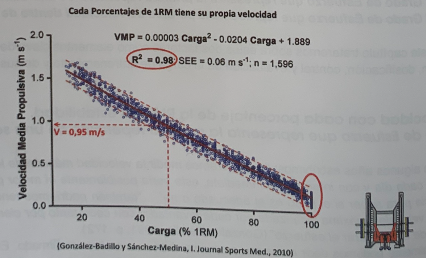
Figure 1. Relationship between the RM percentages and their corresponding mean propulsive velocities. The 1596 data from 176 subjects are practically within the De 95% interval, with an R2 of 0.98 and an estimation error of 0.06 (González-Badillo and Sánchez-Medina)

These differences in the speed of the RMs are responsible for the points going slightly above the mean line or below. That is, the speed of each percentage tends to depend on the speed with which the RM was reached. If with the data of figure 1 the average propulsive velocity (VMP) is considered as an independent variable, we obtain an R2= 0.981; an estimation error of 3.56% and the following regression equation %1RM = 8.4326 * VMP2 – 73.501 * VMP + 112.33, where VMP is the mean propulsive velocity.

If we took the VM speed as a reference, not the VMP, the data would be the following: R2 = 0.979; an estimation error of 3.77% and the equation: %1RM = 7.5786 VM2— 75.885 VM + 113.02, where VM is the average speed of the entire route.

These equations make it possible to estimate with considerable precision the percentage represented by any absolute load once the VMP or MV at which it has moved is known, provided that the speed of movement has been the maximum possible for the subject.

It is preferable to take the average propulsive speed as a reference, since it better represents the true performance of each subject, by eliminating from the measurement the braking phase that occurs when the loads are medium or light. But if the speed meter used does not register this speed value, the average speed can be used, but taking into account that the speeds with each percentage will be slightly lower under light and medium loads if MV is measured than if MP is measured.

If the average or average maximum propulsive velocity with which a mass displaces can be measured, by applying these equations we can obtain the percentage of the RM that said mass represents.

Once you know the percentage that a given mass represents, you can estimate the RM at any time without the need to measure it, although knowledge of the RM is not necessary to dose the training or to assess its effect. Unfortunately, there are many “studies” that have been devoted to estimating the RM in some exercises, when really the value of the RM, when talking about the training load, practically and totally loses its “bad” application if we handle it properly the information that the knowledge of the speed of execution offers us.

According to the regression equation shown in figure 1, the average propulsive velocity that would correspond to each percentage of the RM is presented in figure 2.

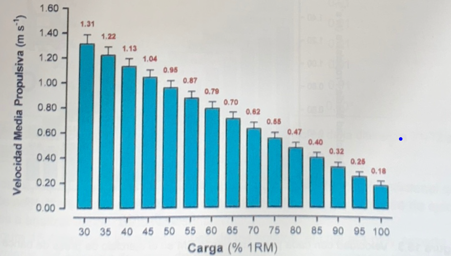
Figure 2. Mean propulsive velocity corresponding to each percentage of the RM in the bench press exercise (González-Badillo & Sánchez-Medina, 2010)

It is very important to verify that the relationship between speed and load is stable, that is, if these values ​​remain very similar when the subjects change their performance, since this is the basis for applying the speed of the first repetition of the exercise. series for reference.

The speed of the first repetition of the series is used to determine with what relative load the subject is training., as well as to determine what has been, and continues to be, the effect of training each day, what has been the evolution of the maximum intensity used each day, and what has been the pre-post training effect…

The training effect is assessed by speed changes at the same absolute loads at any time, which can be before and after a training period or in each of the training sessions. All this constitutes part of the maximum and best information that a coach can have to know what he is doing and improve his training methodology.

The speed of the first repetition of the series is used to determine with what relative load the subject is training.

In this sense, a series of data are provided that serve as a reference to confirm that, indeed, the speed values ​​with each percentage are very stable, even if the performance of the subjects changes and even if the subjects are of a very different level of performance. . A first example of this stability is presented in figure 3, in which the results of two measurements of the speeds are compared with each percentage of the RM in the bench press exercise.

first study: analysis of velocity in the bench press exercise

The values ​​for the year 2010 are the same as those in Figure 2. These values, which were recorded in the years 2006-2007, were obtained with subjects other than the participants in the 2014 study, whose data were recorded in 2013-14, 6-7 years apart. It can be seen that the speed values ​​with each percentage are practically the same. These data help to confirm that the speed with each percentage remains stable, even though the data is obtained with completely different samples.

 

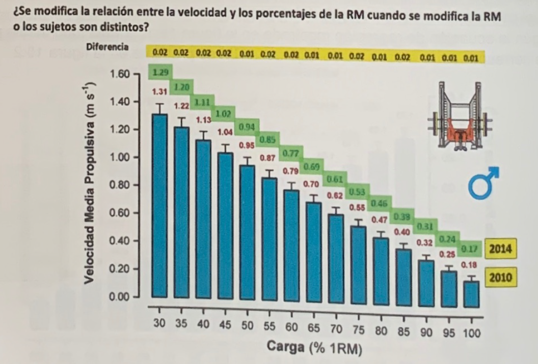
Figure 3. Velocity with each percentage of the RM in the bench press exercise in two different groups of subjects and several years apart in the recording of the data. It can be seen that the differences (upper part of the figure) in the speeds do not exceed 0.02 m-s-1. (Figure by Sánchez-Medina).

Continuing with the examples, in the study by González-Badillo and Sánchez-Medina (2010), carried out with the bench press, it was verified that after a training period of an average of six weeks, 56 subjects, who improved as averaged 9.3% of their RM on the bench press, they kept pretty much the same velocity with each percentage. These data allow us to confirm that not only each percentage of the RM has its own speed, but that this speed is very stable when the performance is modified.

Not only does each percentage of the RM have its own speed, but this speed is very stable when changing performance.

Table 1 shows the average speed values ​​with each percentage before and after the training of the 56 subjects. The maximum difference is 0.01 m*s-1. It should be noted that these subjects trained according to their criteria, without any instruction, which means that the training sessions must have had very different characteristics.

 

 

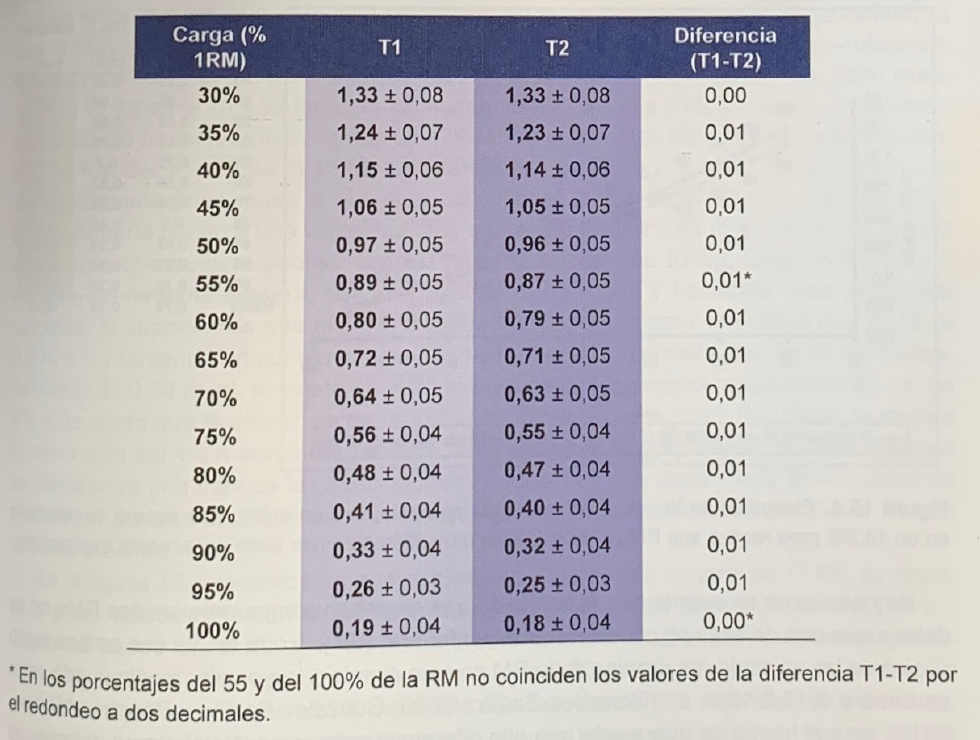
Tabla 1. Mean propulsive velocity and standard deviation with each percentage of the RM in the bench press in 56 subjects before (T1) and after (T2) a training period of 9 weeks on average (González-Badillo & Sánchez-Medina, 2010).

From the individual data of these 56 subjects we can extract additional information that allows us to continue reinforcing the stability of the percentage-speed of execution relationship. Several representative cases are discussed below.

Figure 4 shows the data of one of the subjects, who was very expert in training the bench press exercise, and who clearly improved his 1RM: 14.8%. If we look at the figure of test 2, T2 (red line), apparently, the speeds with each percentage are lower than those of test 1, T1 (blue line). This would go against the hypothesis that holds, but these data are not comparable, so they really do not go against the hypothesis.

The explanation is in the speed with which each RM has been achieved. In T1 the velocity was 0.17 m*s-1, while in T2 it was 0.06 m*s-1 (both values ​​in the red circles at the bottom of the figure). These two RMs cannot be compared, because they have been achieved at clearly different speeds, and, therefore, their speeds with each percentage cannot be compared either: the lower the speed with which the RM is achieved, the lower the speed with each percentage.

If the difference between the speeds of the RMs is equal to 0.03 m*s-1, we can already begin to observe a tendency to be lower than the speeds corresponding to the RM reached at a lower speed, and if the differences are greater than 0.03 m*s-1, the two RMs should no longer be compared.

 

 

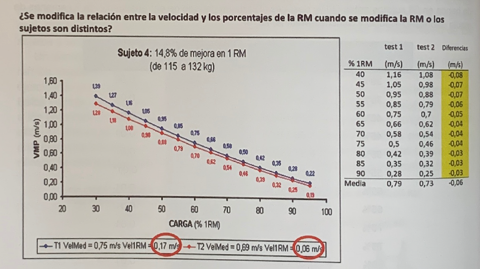
Figure 4. Evolution of speed with each percentage in a subject who exceeds his result by 14.8% but performs his RMs at very different speeds (see text for further explanation).

It must be taken into account that the fact that the two RMs should not be compared is not due to the fact that one of them is considered a “true” RM and the other is not, since both are within the velocities of the RM of this exercise, whose average value may be around 0.17-0.18 m*s-1 (González-Badillo, 2000; González-Badillo and Sánchez-Mediná 2010), but to the fact that there is a high difference between them .

However, despite the fact that in T1 the speed of T2 almost triples, the differences in speeds with each percentage do not exceed, in the worst case (low percentages), 5% of the RM since the difference in speed each 5% is 0.08-0.09 m*s-1, a difference that is not exceeded in any of the percentages calculated, from 30 (0.09 m*s-1 difference) up to 95%.

Conclusions of the first study

As a result of the analysis of this case, at least the following practical applications can be deduced:

1) MRIs whose measurement speeds are greater than 0.03 m*s-1 cannot be compared, although in extreme cases such as the one we are presenting, in which the speed of the MRI is tripled, the effects do not go beyond one difference of 5% of the MR for the same speed of the same subject,

RMs whose measurement speeds are greater than 0.03 m*s-1 cannot be compared,

2) given the high probability that two RM are measured at different speeds, it is not advisable to ever measure the RM (it can be estimated, if necessary for something, as we will see in another section) and

3) only by measuring the speed with which the MR is reached, it is possible to have the necessary information to avoid the errors made with high frequency when measuring this variable.

Here we have to remember that the true RM will never be known, but some RMs can be considered as “true” or representative of the true RM when measured at velocities of their corresponding RM values. The more the measured speed (always higher speeds) deviates from the MR values ​​of an exercise, the more “false” is the RM measurement. This, once again, can only be known if the speed with which the exercise is performed is measured.

The errors to which we refer in the practical application 3) refer to the fact that most of the changes, such as the improvement or worsening of the results observed when measuring 1RM, are false, because if a subject, for example (it is a case real), lifts 82 kg in T1 and 92 kg in T2, it can be concluded after doing the calculations, that the subject has improved his mark by 12%.

But if one takes into account that this subject did the MRI of T1 at 0.33 m*s-1 (real data) and that of T2 at 0.2 m*s-1, the conclusion is false, because if the subject could have done the MRI at T2 at 0.2 m*s-1, it could also have been done at a very similar speed (0.2 + 0.02 m*s-1) at T1.

This would mean that he could have lifted a weight greater than 82 kg, then the improvement has not been, by any means, 12%. As an example, and making a few small calculations, if we suppose that the T1 would have done it at the same speed as the T2, at 0.2 m*s-1, and taking into account that every 5% the speed change is 0.08 m*s-1, the subject in T1 would have lifted approximately 88 kg, 8% more, given that the difference between T1 and T2 is 0.13 m*s-1.

Therefore, the improvement would have been approximately 4-5%, far from the apparent 12%. This example shows one more of the important applications that measure the speed of my execution has, although this application is better not to use it, because the RM should never be measured.

second study

A new example is shown in Figure 5. This subject improved his result by 11.8% and the velocities with the MRI presented a small difference of 0.02 m*s-1. As can be seen, the velocities with each percentage remained practically stable, with a maximum difference of 0.02 m*s-1, that is, the equivalent of a maximum difference of 1.25% of the RM with respect to T1.

Also, in this case, the speed in all percentages tended to increase slightly, so it could be said that the subject slightly improved (because the change can only be very small) his strength deficit. This slight improvement in speed can be explained because the subject, after his experience in doing the tests, decided to train by performing each repetition at the maximum speed possible, when previously he did it slowly voluntarily.

Therefore, it is confirmed that despite a considerable improvement of almost 12% (in this case we can say that it is real), the speeds with each percentage remain stable.

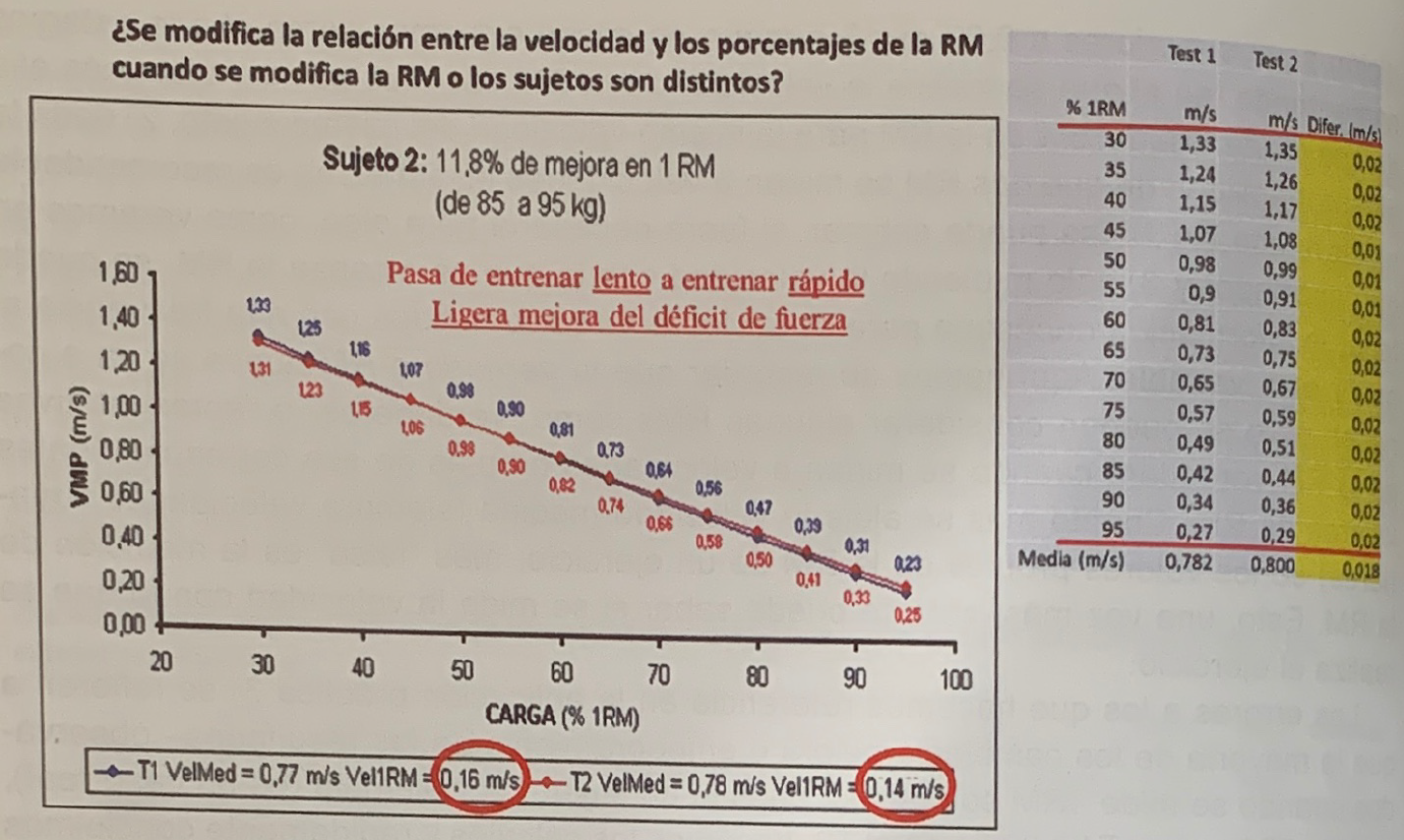
Figure 5. Evolution of speed with each percentage in a subject who exceeds his result by 11.8% and performs his RMs at very similar speeds

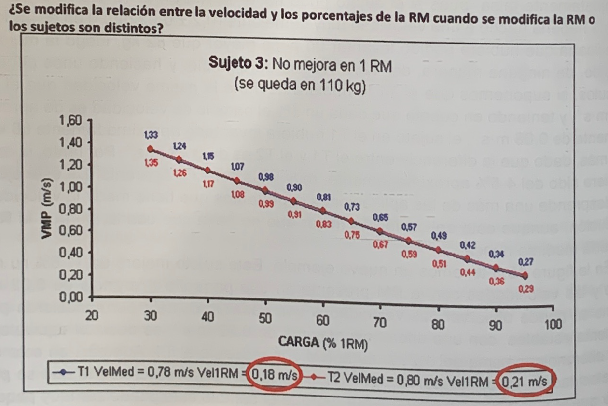
Figure 6. Evolution of speed with each percentage in a subject who does not exceed his result and performs his RMs at very similar speeds

Figure 6 shows an example of a subject who did not improve his result and that the speeds with each percentage were practically the same in both tests, although T2 was performed at a speed of 0.03 m*s-1 higher than the from T1.

But, precisely, this small speed difference could explain, on the one hand, why the speeds in T2 are minimally higher (0.01-0.2 m*s-1), and on the other, that it really cannot be said that the subject It did not improve its performance at all, since it improved speed by 0.03 m*s-1 with the same load (110 kg). This assessment can only be done if the speed of execution is measured

Figure 7 shows the case of a subject who improved his RM by 7.9%, who performed his two RMs at the same speed, but the speed with each percentage up to 75% of the RM tended to decrease. This was the only case, out of 56, that departed from what we have been maintaining. But when consulting the subject about his way of training, he stated that he trained slowly voluntarily.

Training slowly voluntarily may tend to proportionally decrease performance with loads moving at high speed and thus increase the strength deficit under these loads.

This way of training may tend to proportionally decrease performance with loads that are moved at high speed and thus increase the strength deficit in the face of these loads. Despite this circumstance, it can be observed that the decrease in speed with light loads did not exceed 0.06 m*s-1, which means that, in the worst case, the maximum difference in speed with each percentage in T2 with respect to T1 it was equivalent to 3.7% of the OR.

Figure 7, Evolution of speed with each percentage in a subject who exceeds his result by 7.9% and performs his RMs at the same speed.

In Table 2, made up of two groups of data, with a total of 20 subjects (the first 20, by random order, in the list of 56 subjects who repeated the tests) we can see the speed at which they reached their RMs. in tests 1 and 2, the average speed of the percentages from 40 to 90% of the RM, the maximum and the minimum difference obtained in the set of these percentages and the change in performance.

It is observed that the average speed from 40 to 90% follows the same trend as the difference between the speeds of the RMs. Only in the cases of JG and PC subjects, the maximum difference in some percentage is equivalent to a 5% difference with respect to the RM.

It can be seen that there are 12 cases of improvements ranging from 8.3 to 21.23% with an average of 13.9%, in which the maximum difference in speed with the percentages from 40 to 90% is 0.05 m*s-1 in the two subjects mentioned above (JG and PC), one case with 0.04 m*s-1 (V) and the rest with 0.03 m*s-1 or less. This data set again reinforces the stability of the speed of each percentage, even if there are important changes in the performance of the RM.

 

 

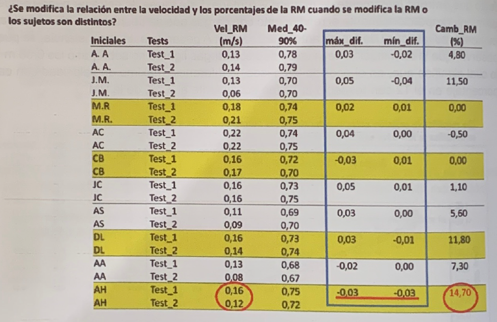
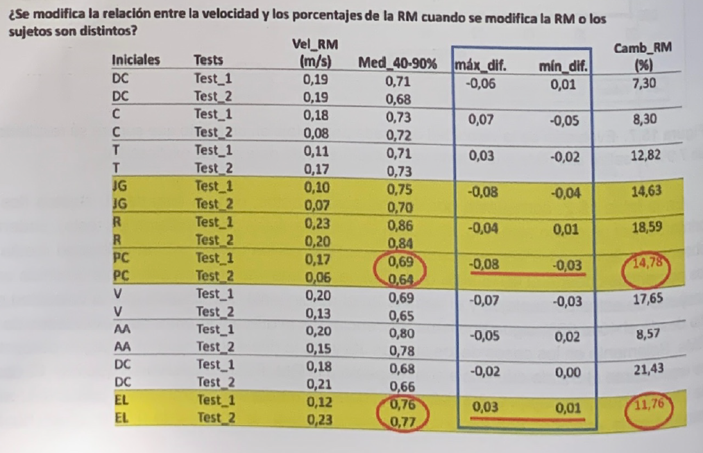
Table 2 Velocity values ​​with the RM (vel_RM), average velocity of the velocities with the percentages between 40 and 90%, maximum (max_diff), and minimum (min_diff) velocity difference with each percentage between tests 1 and 2 and change in performance (Change_RM) of the first 20 subjects in the list of 56 who repeated the tests.

Table 3 shows the speeds with the RMs, mean speeds from 40 to 90% of the RMs, differences in the speed with the RM and the differences between the mean speeds with the set of percentages in two tests for the same subjects included in Table 2. Taking the set of data included in the yellow columns, it is possible to calculate the relationship between the differences in the speed of the MRI and the differences in the average speed of

 

 

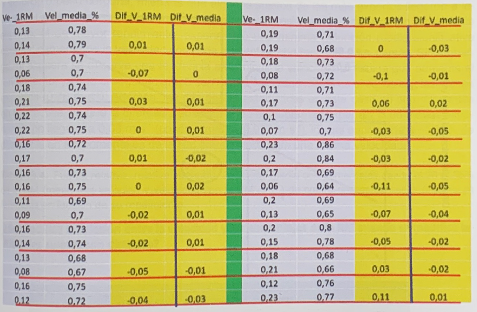
Tabla 3. Speeds with the RMs (Ve_1RM), mean speeds of the percentages from 40 to 90% of the RMs (Vel_mean_%), differences in speed with the RM (Dif_V_1RM) and the differences between the mean speeds with the set of percentages in the two tests (Dif_V_mean) of the same subjects included in Table 2.

Figure 8 shows the relationship between the differences in the speed with which the RMs were achieved (axis X) and the differences in the mean speed in the percentages of the RM from 40 to 90% (axis Y).

It can be seen that 12 of the 20 cases are found in the positive quadrants of the coordinate axes, which are the ones that correspond to the trend that indicates that the speed of the MRI determines the speed with each percentage, that is, the higher is the speed of the RM the greater the speed tends to be with each percentage.

There are three cases in which the velocities with the MRI were the same (points that coincide with the Y axis) and the velocities with the percentages changed minimally, between 0.03 and 0.02 m*s-1.

A case in which, having produced a decrease in the speed of the MRI in T2 by about 0.07 m*s-1, the average speed of the percentages was identical (point located on the X axis). This case can be considered as an example of a subject improving his strength deficit: although a lower MR speed should correspond to a slightly lower speed with each percentage, the subject maintained a speed.

There are two cases in the lower negative quadrant in which, having slightly increased the speed with the MR around 0.02 m*s-1, the speed with the percentages decreased by 0.02 m*s-1, which suggests that it was produced a minimal increase in strength deficit.

Finally, there is a case in the upper negative quadrant in which a subject who performed his MRI speed at a slower speed (0.02 m*s-1) at T2 slightly increased speed with percentages (0, 01 m*s-1).

As can be deduced, the stability of the speed with each percentage is ratified. The changes are minimal and the trend between the speed with the RM and the speed with each percentage is fulfilled in a remarkable way.

 

 

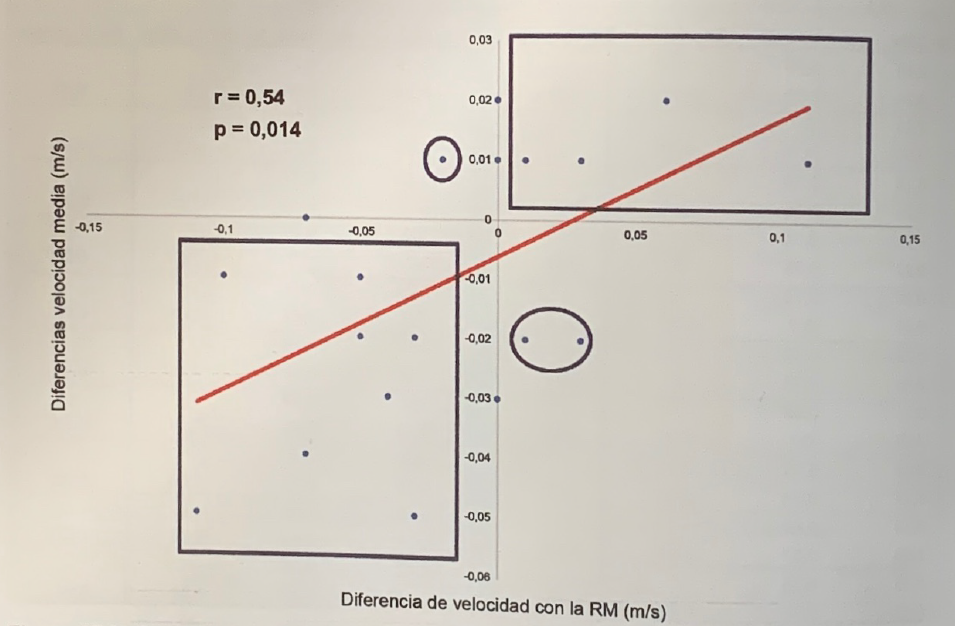
Figure 8. Relationship between the differences in the speed with which the RMs were achieved (axis X) and the differences in the mean speed in the percentages of the RM from 40 to 90% (axis Y).

It must be taken into account that the subjects cannot behave like perfect “machines”, but that they respond in a way that is not exactly the same before a series of progressive loads when trying to perform a 1RM test. This means that under absolute load the performance is not exactly the same as under the immediately higher absolute load.

That is to say, if a subject achieves a certain speed at an absolute load, not always at the load immediately above, which will represent a certain percentage increase, he will respond by reaching exactly the speed that would correspond to that percentage increase in load. This can cause the subject’s force or load-velocity curve to adjust more or less to his true performance capacity, giving rise to small deviations from the model that represents the population to which the subject belongs.

Does performance level affect speed?

To continue adding elements to confirm the stability of the speed with each percentage, it could be assessed whether the speed with each percentage is similar or not between people with different levels of performance.

From the results of the study it can be deduced that, indeed, the speed with each percentage is very similar between people with a very different level of performance. By dividing the group of 176 cases into four groups based on their relative MR (RM * body weight-1), the mean speeds from 30 to 95% of the RM were 0.76, 0.77, 0.77 and 0.73 m*s- 1 (table 4), in this order, from the group with the lowest performance to the most expert group, respectively.

Therefore, the average speed is almost the same despite the performance increase considerably. Consider that the subjects with the lowest performance did not get to lift a weight equivalent to their own body weight in the bench press, while some of the most expert subjects came to lift twice their body weight or approached this mark.

Less performing subjects failed to bench press their own body weight, while some of the most experienced subjects lifted twice their body weight

Only the highly expert group, the one with the highest performance, experienced a minimal statistically significant average reduction in speed with each percentage compared to the others. However, a tendency to decrease speed is not even observed as performance increases, since the second group with the lowest average speed is that of the less expert subjects (0.76 m*s-1).

In addition, the statistical differences in this case are not relevant in practice, since the absolute difference between the most expert group and the least experienced group is not even 0.03 m*s-1 (specifically, 0.027 m*s- 1), which would be equivalent to a -1.69% difference in the RM percentages between the two for the same speed.

 

 

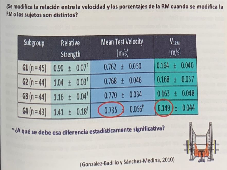
Tabla 4. Relative strength (relative strength), mean speed with percentages from 30 to 95% of the RM (mean test velocity) and speed with the RM (V1RM) of four groups of cases (subgroup) formed according to their performance.

However, if these results are analyzed in greater depth, it is concluded that these differences are not real. Responding to the question formulated in the lower part of Table 4, the apparent lower speed with each percentage of the most expert group is due to the fact that the average speed with which the components of this group reach their RM is slightly less than that of the others (0.045 m*s-1 with respect to the group with the lowest performance, and 0.019 and 0.014 m*s-1 for the other two groups).

This fact causes that, necessarily, the speed with each percentage tends to be lower, which comes to ratify, once again, what has already been revealed previously. Thus, the slight decrease in speed with each percentage of the top performing group in the bench press exercise is due to the tendency to decrease speed with RM in extremely expert subjects.

It is reasonable to accept that these subjects are able to make the most of their own strength potential, because they have more confidence in their possibilities and better technique when executing the exercise. It should be noted that, given the characteristics of the subjects in this study, the generalization of these data leads us to be able to apply them to the entire population, since in the group there are subjects who lift from less than 90% of their body weight up to subjects lifting twice their body weight.

This means that any young person practicing any sport or simply using strength training can be included here. Therefore, this is one of the few exercises that would really allow us to assess our strength-speed “profile”.

If we execute the exercise well, we will be able to know to what extent our performance in this exercise is in the average of the population in terms of speed with each percentage, if it is slightly above or if it is slightly below, or even if it is below. above or below in some areas and not in others of the force-velocity curve or not.

However, to make these assessments, one must also take into account the speed at which MR is reached. But the stability in the relationship between the percentages of the RM and their corresponding speeds also occurs in any exercise in which the measurements have been made well.

Table 5 shows the data corresponding to the complete squat exercise. The group consisted of 80 subjects. The differences in performance are important, from 93 to 126 kg on average, with coefficients of variation from 12 to 18%, and some subjects lifting more than twice their body weight (1.57 to 2.17 range in the highest performing group).

Therefore, we can admit that it is a sample that includes a range of performance in which a wide population of athletes can be found.

the average speed of all the percentages is practically the same

However, the mean speed of the set of percentages (mean test velocity) is practically the same (0.873, 0.867 and 0.865 m*s-1) The speeds with the percentage examples included in the table are practically the same in the three groups , existing between 0.01 and 0.02 m*s-1 as a maximum difference. The MRI speed of each group is practically the same as that of the others, and the same as that indicated in the year 2000 (González-Badillo, 2000). No significant difference is observed in any of these speed values.

 

 

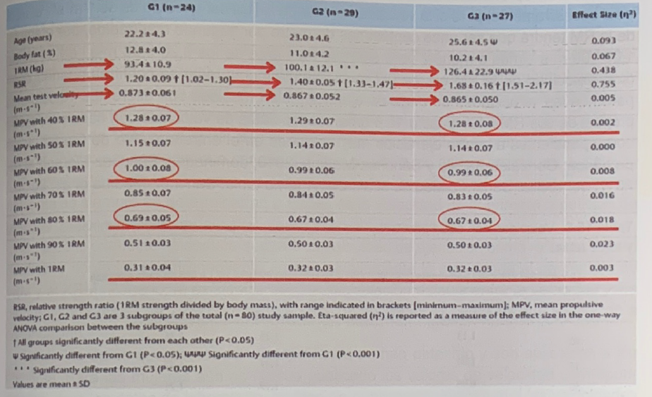
Tabla 5. Comparison of the mean speeds of the tests with percentages from 30 to 95% of RM (mean test velocity), mean propulsive velocity with different percentages (MPV), mean propulsive velocity with RM (MPV with 1RM) in three groups formed based on their vative performance with respect to body weight (RSR) in the full squat test. The effect size is represented by the “eta” statistic (effect size n2) (Sánchez-Medina et al., 2017).

Therefore, In an exercise as different from the bench press as the squat, the stability of the speed is confirmed with each percentage, although the performance of the subjects is very different. It has been indicated that the speed with each percentage is dependent on the speed with which RM is reached. This tendency has been verified when analyzing the different examples of performance with the bench press exercise.

Although this tendency not only occurs in the same exercise when the speed of the RM changes due to its faulty measurement, but naturally also occurs between the different exercises, because each exercise has its own speed, and different from that of the others. , from his RM (González-Badillo, 2000).

In this article, published with data recorded in the 1990s, it was already commented that the speed with 40% of the RM of the bench press was 1.15 m*s-1, which differs in only two hundredths of a m*s-1 of the current data (1.13 m*s-1), and the squat had a speed of 0.93 m*s-1′ with 64.3% of the RM, practically the same speed that is currently proposed (0.92 m*s-1 with 95%. see table 6).

each exercise has its own speed, and different from the others

Likewise, it was confirmed that the speed with each percentage depended on the speed of the RM, because the snatch, with an average RM speed of 1.04, the speed of 1.15 m*s-1 was obtained with 91% of the RM, while, as we have indicated, this same speed of 1.15 m*s-1 with the bench press belonged to 40% of the RM, with a speed of his RM of 0.2 m* s-1. The same was the case with the power clean: 1.09 m*s-1 for 87% of the RM and a velocity of his RM of 0.9 m*s-1.

The fact that the speed with each percentage depends on the speed of the RM is so evident that we can say that it is “truth”, although this does not prevent someone from occasionally questioning it.

It is evident that if the speed of the RM of an exercise is, for example, 0.2 m*s-1, the speed of 95% of the RM of that exercise should be approximately 0.26-0.28 m *s-1, and 90% should be 0.32-0.34 m*s-1 and so on, but if the RM speed of the exercise is 1 m*s-1, 95% of the MRI will have to be a few hundredths of a meter per second faster, for example, 1.08-09 m*s-1, more or less, but always very far from 0.26-0.28 m*s- 1 of the exercise whose MRI velocity was 0.2 m*s-1.

Naturally, this is confirmed when the speeds of different well-measured exercises are compared with different speeds of their own RMs.

Table 6 shows the speed data with each percentage corresponding to four very common exercises in strength training (bench press: González-Badillo and Sánchez-Medina, 2010; pull-ups: Sánchez-Moreno et al., 2017; squat : Sánchez-Medina et al., 2017; rowing table: Sánchez-Medina et al., 2014).

 

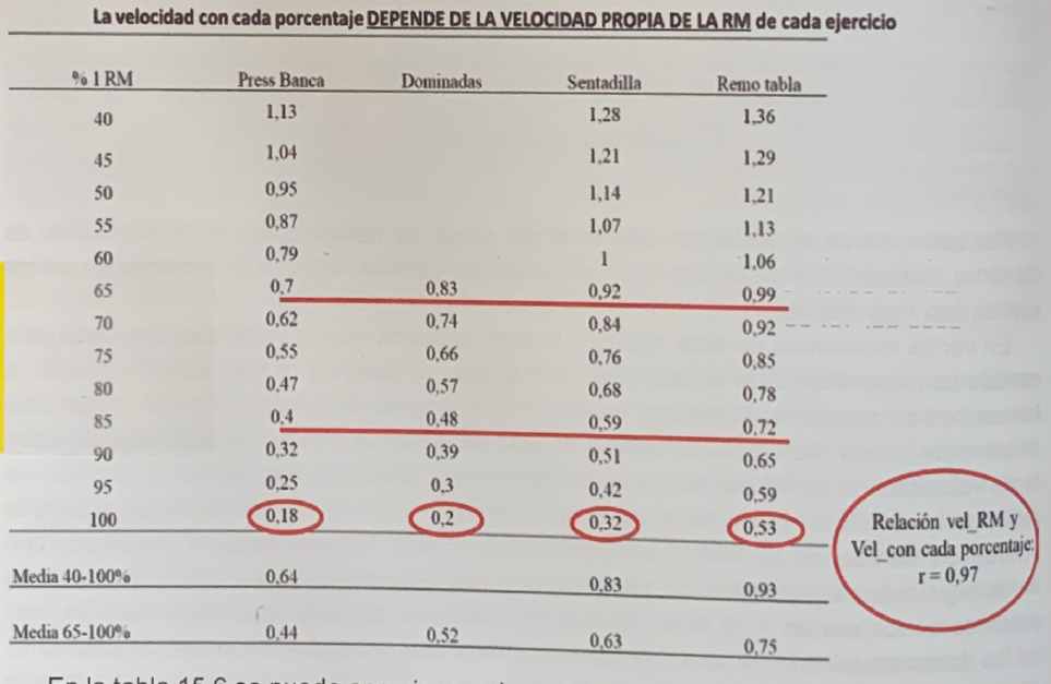
Tabla 15.6. Speed ​​with each percentage in the bench press, pull-ups, squats and plank rows.

Table 6 shows that the speed values ​​of each percentage increase as the speeds of the RMs increase. The relationship between the speeds of the RMs and the average speed of all the percentages from 65% to 100% is almost perfect (r= 0.97; p < 0.05).

It is very relevant that with only 4 pairs of data the correlation is statistically significant. Therefore, it is confirmed that, indeed, the speed with each percentage is dependent on the speed of the RM of the exercise, as well as the differences in the speed of measurement of the RM when it is measured more than once within each exercise. .

As a synthesis of all the above, it is confirmed that training can be controlled through the speed of the first repetition in the series, provided that it is done at the maximum speed possible, and this is based on the fact that we can start from the assumption that if Although the value of 1RM can change between different days, the speed at which each percentage of the RM is performed is very stable.

It is confirmed that the training can be controlled through the speed of the first repetition in the series as long as it is done at the maximum possible speed.

Therefore, speed control can inform us with high precision about what real percentage or what effort is being made at each moment. Therefore the own speed of each percentage of 1RM determines the real effort. This means that the speed of the first repetition of a set determines the degree of effort that the load represents.

Thus, the training load (mass) can be determined by the speed of the first repetition. If this is so, what should be programmed is not the percentage of 1RM or an XRM, but the speed of execution of the first repetition of the series. Note: for convenience or to be more intuitive, it could be programmed by means of the RM percentages, but the absolute loads (masses) that correspond to those of the percentages would always be determined through the speed of the first repetition of the RM. series, not by the result of the arithmetic calculation of the percentage.

conclusions

From all of the above, it can be deduced that using the speed of execution as a reference to dose and control the training far exceeds what the percentage of 1Rm and XRM contributes. Therefore, the existence of a high stable relationship between speed and the different percentages of 1RM allows a series of applications such as those indicated below.

All the data that have been provided have been obtained and are applicable to men. For women, the corresponding speed values ​​have not yet been published, but laboratory data, in the publication phase, indicate that the speeds with each percentage are practically the same with women from a relative intensity of 45-50%, reducing approximately at 0.03, 0.04 and 0.06 m*s-1 with the intensities of 40, 35 and 30% of the MR, respectively.

the speeds with each percentage are practically the same with women

Knowing the speed of the first repetition (speed with each percentage) allows:

• Evaluate the strength of a subject without the need to perform a 1RM test or an XRM or nRM test at any time.
• Determine with high precision what real percentage the subject is using as soon as he performs, at the maximum speed possible, the first repetition with a determined absolute load.
• Estimate / measure the improvement or not in performance EVERY DAY without the need to perform any test, simply by measuring the speed with which an absolute load moves. If, for example, the difference in speed between 70 and 75% of the RM of a specific exercise is 0.08 m*s-1, when the subject increases the speed by 0.08m*s-1, with the same load absolute, there is a very high probability, almost 100% that the load with which you train represents 5% less intensity. Naturally, if what is produced is a loss of speed before the same absolute load (kg), we can be quite sure that the subject is below his previous performance, and in a proportion proportional to the loss of speed before the same load. absolute load.
• The measurement of the speed of the first repetition on a daily basis, just week before and after the training allows:
  • Know the degree and time of adaptation individually.
  • Discover the degree of disparity of the adaptive responses.
  • Check the effect of improving strength on other types of performance trained or not.

Regarding the speed of the MRI, it can be concluded that:

• The only way to be able to consider an MR as “true” or false is to measure the speed with which it is achieved.
• Two MR values ​​of the same subject cannot be compared if the values ​​of the speeds with which they have been measured are not the same or very similar.
• If the speeds at which the pre-post training RMs have been measured are different, with differences greater than or equal to 0.03 m*s-1, these RMs are not equivalent, so comparing the values ​​of the RMs (weights raised) pre-post training would lead to erroneous decisions, considering that there have been some changes in strength (in the MRI) that are not real.
• In addition, the speeds with each percentage would appear to be different, without meaning that they really are.

Regarding the assessment of the effect of training, it is concluded that:

• MRI is not necessary and should never be measured.
• The best procedure for assessing the training effect is to re-measure the speed reached at the same absolute loads that were measured in the initial test.
• This procedure is the most coherent and precise, since the effect of strength training is measured by the change in speed at the same absolute load or, as already indicated, the assessment of the training effect through changes in MR. , even in the not very probable assumption that the speeds with which the RMs are measured are the same or very similar, it would only inform us about the effect of the training before the maximum load (RM), but not before other lower loads

Other apps:

• Use strength training with all subjects, from children to the most advanced athletes or adults and older people who want to improve their health, without the need to do maximum effort tests (1RM, or XRM, for example) in any case.

The authors’ proposal, therefore, is that the mean propulsive velocity of the first repetition should always be used to program, dose and evaluate the training load and the performance of the subject.